Project Two - Educationally Influenced: Predicting the Academic Success Rates of Students in Cyprus
I. Introduction
As someone who always wanted to go into teaching, I have always been fascinated by the diverse makeups that classrooms bring together, there is perhaps not such a more heterogenous space in society that is so commonly available. The magic of teaching for me is that every single student carries their own dreams, aspirations, and motivations—and crucially from a pedagogical perspective, their own background knowledge. It is miraculously up the lecturer at hand to convey knowledge at a carefully-sculpted rate, depth, and breadth that sufficiently engages all students without leaving those behind that are clearly struggling with the ideas or stultifying those that clearly have sufficiently grasped the material and are ready for a greater challenge (or perhaps, most frustratingly for a teacher, students who simply do not care). In an ideal scenario, teachers could analyze the background and study habits of each student, develop a personalized plan that either curbs potential barricades to academic success or encourages characteristics that underpin in, and reap the success of a spirited, confident, and well-educated classroom.
Where such a ideality was previously limited to the imaginations of educators, like many things in the modern-day, it can increasingly become a reality with the rise of machine learning and artificial intelligence systems. Ethical considerations at bay (because they certainly are quite a few), the ability to input an entire student’s demographics, personality, and interests into an algorithm and immediately how to best get that student to learn and critically, enjoy that learning, is maybe one of the most altruistic and revolutionary innovations brought upon this digital revolution.
Thus, the following project delves into a fundamental question: Which features of a student are most correlated with academic success and how can we utilize these features to predict which grades they will achieve in their studies?. Forecasting such an outcome takes more than just analyzing a student’s study hours and class attendance; it demands at through look at their socioeconomic status, their familial circumstances, and their actions before, during, and after class. Only with such a holistic view can we even begin giving justice to this socially-essential inquiry.
Where did this data even come from?
Courtesy of the amazing UC Irvine Machine Learning Repository is a dataset released in 2023 about Engineering and Educational Science students attending Near East University in Cyprus. The best part of this dataset is that was utilized to support findings in a paper named Student Performance Classification Using Artificial Intelligence Techniques, so while doing my analysis, I can compare the results to actual researchers that completed a very similar task (and see if I can beat them, probably not though).
There are not an incredible amount of samples in the dataset (only 145), but quite a few features for each student that include:
- Parental Education & Other Familial Information
- Study Habits (amount of hours, amount of scientific & non-scientific literature read, how often a student took notes in class)
- Attendance to various academic-related events and also classes
- Preparation before particular exams
- The student’s academic performance (both in GPA and grade)
If you’d prefer to download this notebook, just press here.
II. Pre-Processing and Visualizing the Data
We can load in our dataframe like always do to get started:
edu_df: pd.DataFrame = pd.read_csv('./datasets/cyprus_education_dataset.csv')
Let’s take a peek at our first ten rows:
| STUDENT ID | 1 | 2 | 3 | ... | 29 | 30 | COURSE ID | GRADE | |
|---|---|---|---|---|---|---|---|---|---|
| 0 | STUDENT1 | 2 | 2 | 3 | ... | 1 | 1 | 1 | 1 |
| 1 | STUDENT2 | 2 | 2 | 3 | ... | 2 | 3 | 1 | 1 |
| 2 | STUDENT3 | 2 | 2 | 2 | ... | 2 | 2 | 1 | 1 |
| 3 | STUDENT4 | 1 | 1 | 1 | ... | 3 | 2 | 1 | 1 |
| ... | ... | ... | ... | ... | ... | ... | ... | ... | ... |
| 141 | STUDENT142 | 1 | 1 | 2 | ... | 5 | 3 | 9 | 5 |
| 142 | STUDENT143 | 1 | 1 | 1 | ... | 4 | 3 | 9 | 1 |
| 143 | STUDENT144 | 2 | 1 | 2 | ... | 5 | 3 | 9 | 4 |
| 144 | STUDENT145 | 1 | 1 | 1 | ... | 5 | 4 | 9 | 3 |
145 rows × 33 columns (total)
We can see that all of the column names and values are numerical, which is super helpful perhaps for a machine learning model but not so helpful for us mere human non-models. So, my first pre-processing step was simply renaming all the columns to the values they actually are so you (and I) can figure out what they are a little bit more.
# The columns are just numbers, so I am replacing them with their actual values
col_names: list = ['Age', 'Sex', 'School Type', 'Scholarship Percentage', 'Additional Work', 'Regular Art/Sports', 'Has Partner', 'Total Salary', 'Transportation Medium', 'Accommodation Type', "Mother's Education", "Father's Education", "Number of Sisters / Brothers", "Parental Status", "Mother's Occupation", "Father's Occupation", "Weekly Study Hours", "Reading frequency (non-scientific books/journals)", "Reading frequency (scientific books/journals)", "Attendance to department seminars / conferences", "Impact of projects / activities on your success", "Attendance to Classes", "Preparation to midterm exam 1", "Preparation to midterm exams 2", "Taking notes in classes", "Listening in classes", "Discussion improves my interest and success in the course", "Flip-classroom", "Cumulative GPA last semester", "Expected GPA at graduation", "Course ID", "Output Grade", "Student ID"]
edu_df.columns = col_names
Now we have:
| Age | Sex | School Type | Scholarship Percentage | ... | Expected GPA at graduation | Course ID | Output Grade | Student ID | |
|---|---|---|---|---|---|---|---|---|---|
| 0 | STUDENT1 | 2 | 2 | 3 | ... | 1 | 1 | 1 | 1 |
| 1 | STUDENT2 | 2 | 2 | 3 | ... | 2 | 3 | 1 | 1 |
| 2 | STUDENT3 | 2 | 2 | 2 | ... | 2 | 2 | 1 | 1 |
| 3 | STUDENT4 | 1 | 1 | 1 | ... | 3 | 2 | 1 | 1 |
| ... | ... | ... | ... | ... | ... | ... | ... | ... | ... |
| 141 | STUDENT142 | 1 | 1 | 2 | ... | 5 | 3 | 9 | 5 |
| 142 | STUDENT143 | 1 | 1 | 1 | ... | 4 | 3 | 9 | 1 |
| 143 | STUDENT144 | 2 | 1 | 2 | ... | 5 | 3 | 9 | 4 |
| 144 | STUDENT145 | 1 | 1 | 1 | ... | 5 | 4 | 9 | 3 |
145 rows × 33 columns (total)
Much better! Our values are still a bit vague (what is a 3 Scholarship Percentage), but we can modify each column as necessary for our visualization step. Now we can move on to seeing the first step actually pre-processing our data: verifying if there any null values.
print(f'The number of NaN values per column in our dataset: \n {edu_df.isna().sum().sort_values(ascending=False)}')
The number of NaN values per column in our dataset:
 Age                       0
Sex                       0
School Type               0
Scholarship Percentage    0
Additional Work           0
Regular Art/Sports        0
Has Partner               0
Total Salary              0
Transportation Medium     0
Accommodation Type        0
dtype: int64
Ah! Perfect! Super unrealistic but UCI archive did actually tell us there are no missing values within this dataset, making it super easy to work with. That is likely the result of this being a very small and manually-collected collection process, so many missing values were likely handled long ago (also the fact that the original researchers would deal with them as part of their own ML work before releasing it to the public!).
However, we do not have zero pre-processing to do (ah, I wish). There is still quite a bit work we need to do if you want to make sense of all of this data and ensure that we are identifying the most pertinent features and the best model to identify trends within those features. If we are are trying to predict student outcomes, I think a good first step is to see what outcomes we are dealing with; in other words, model the distribution of grades and GPA that this particular dataset contains.
However, in order to do that, we must do some interesting conversions as the grading system is currently numerically encoded and those numbers convert to the specific grading system used at NEU University in Cyprus, which must be further converted to ECTS grades and finally US-scale grades. To accomplish this, I used a resource provided by NEU to convert their grading system to ECTS and then utilized the most logical grade from the ECTS system based upon the equivalent US grade # Let’s change the grades so they are a lit bit more interpretable by us [1]
grades_mapping: dict = {0: 'F', 1: 'D', 2: 'C-', 3: 'C+', 4: 'B', 5: 'B-', 6: 'B+', 7: 'A-', 8: 'A', 9: 'A+'}

# Convert the numerical Cyprus grading system grades to American Letter Grades
edu_df['Output Grade'] = edu_df['Output Grade'].map(grades_mapping)

# Make these letter grades ordinal
edu_df['Output Grade'] = pd.Categorical(
    edu_df['Output Grade'],
    categories=grades_mapping.values(),
    ordered=True)

edu_df['Output Grade']
From there, I used my favorite visualization package, plotly to make two graphs: One of the grade distribution of all the students within our training dataset and one of the expected GPA distribution of all the students.
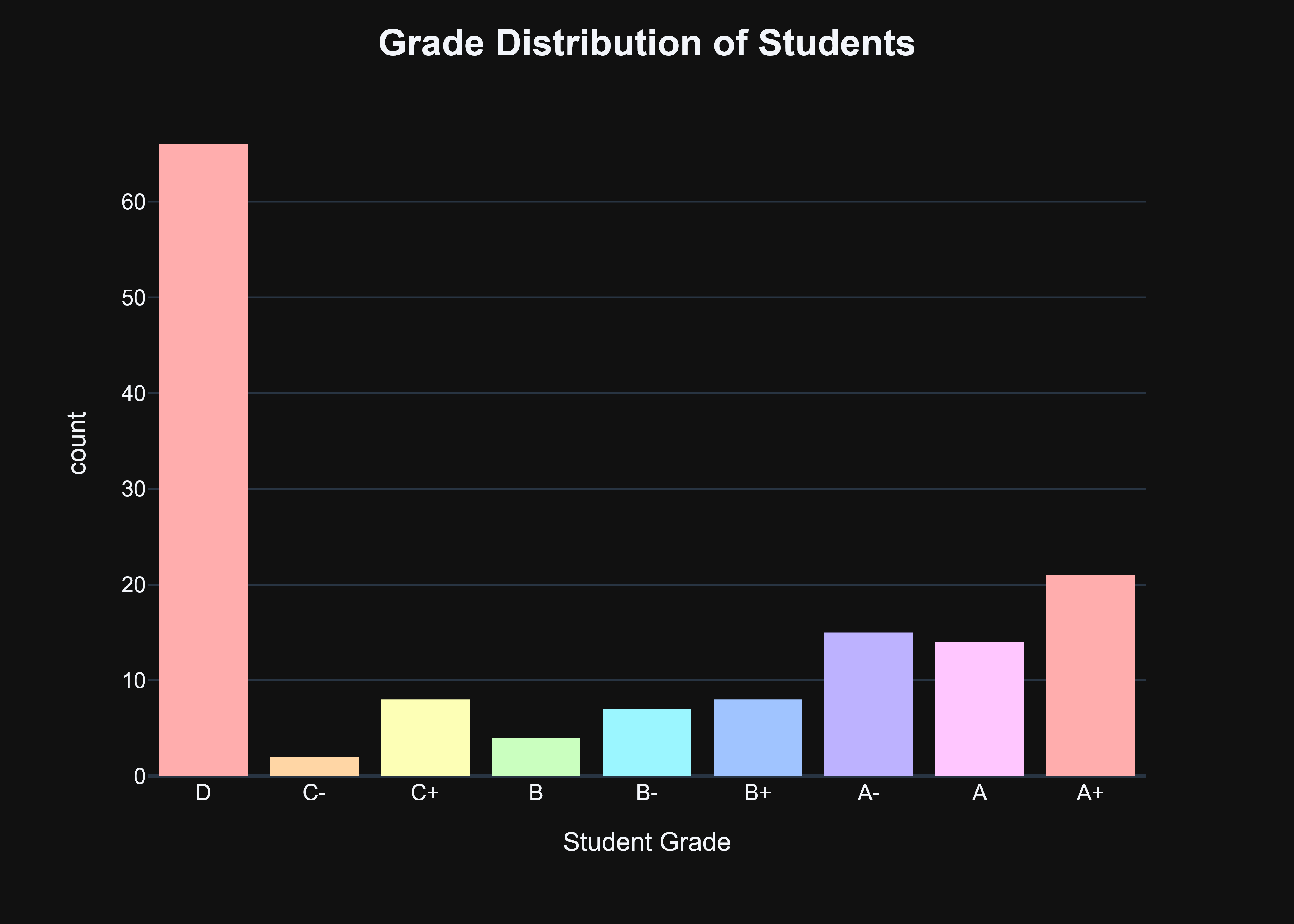
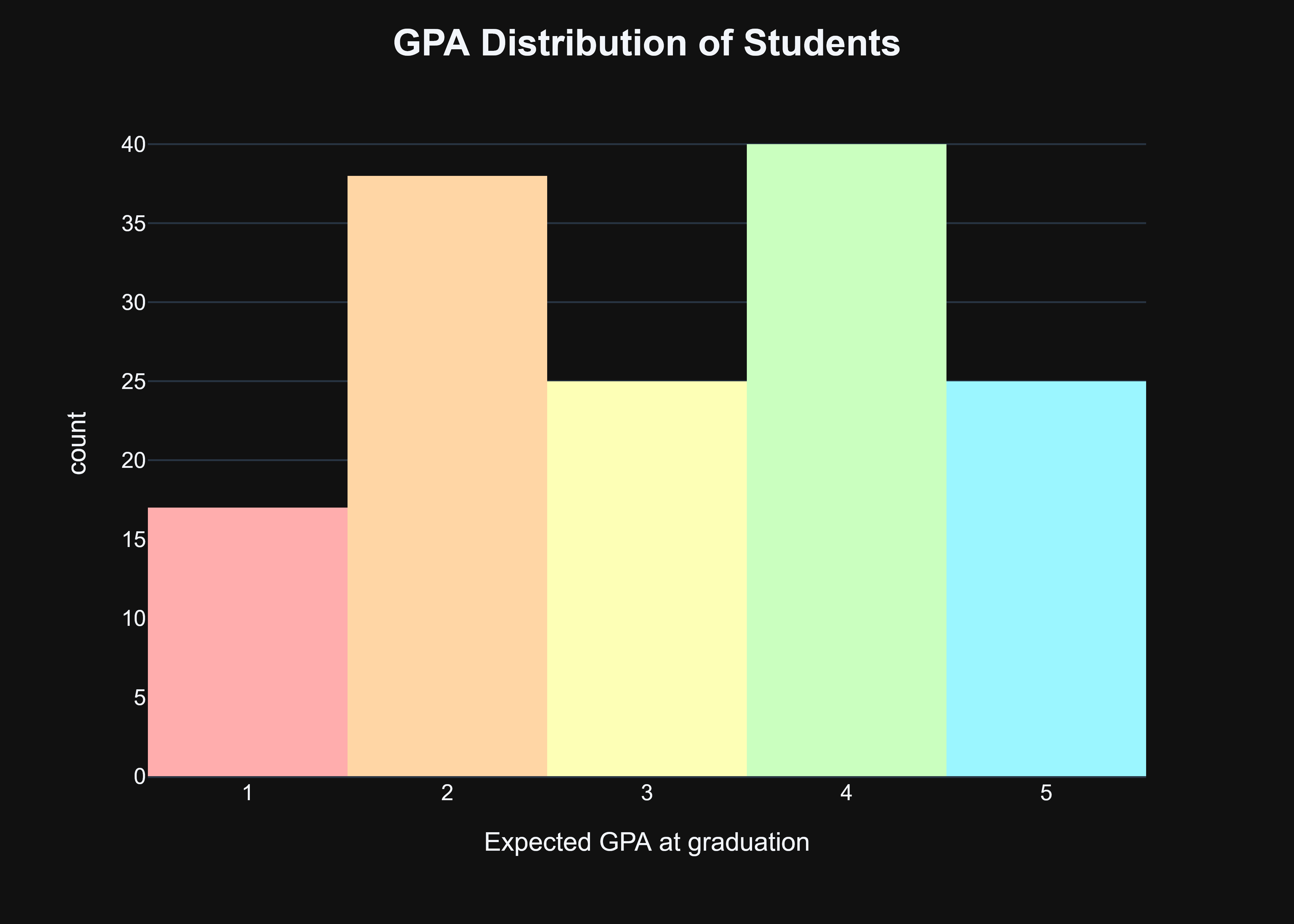
Now, that might look a bit concerning given that most students do not have a very good grade, however, I view it as a potential benefit. It shows that there are a very select amount of students that are high-performing in this given survey and analyzing their patterns, situation, and demographics especially can provide a lot of insight into the background of successful students.
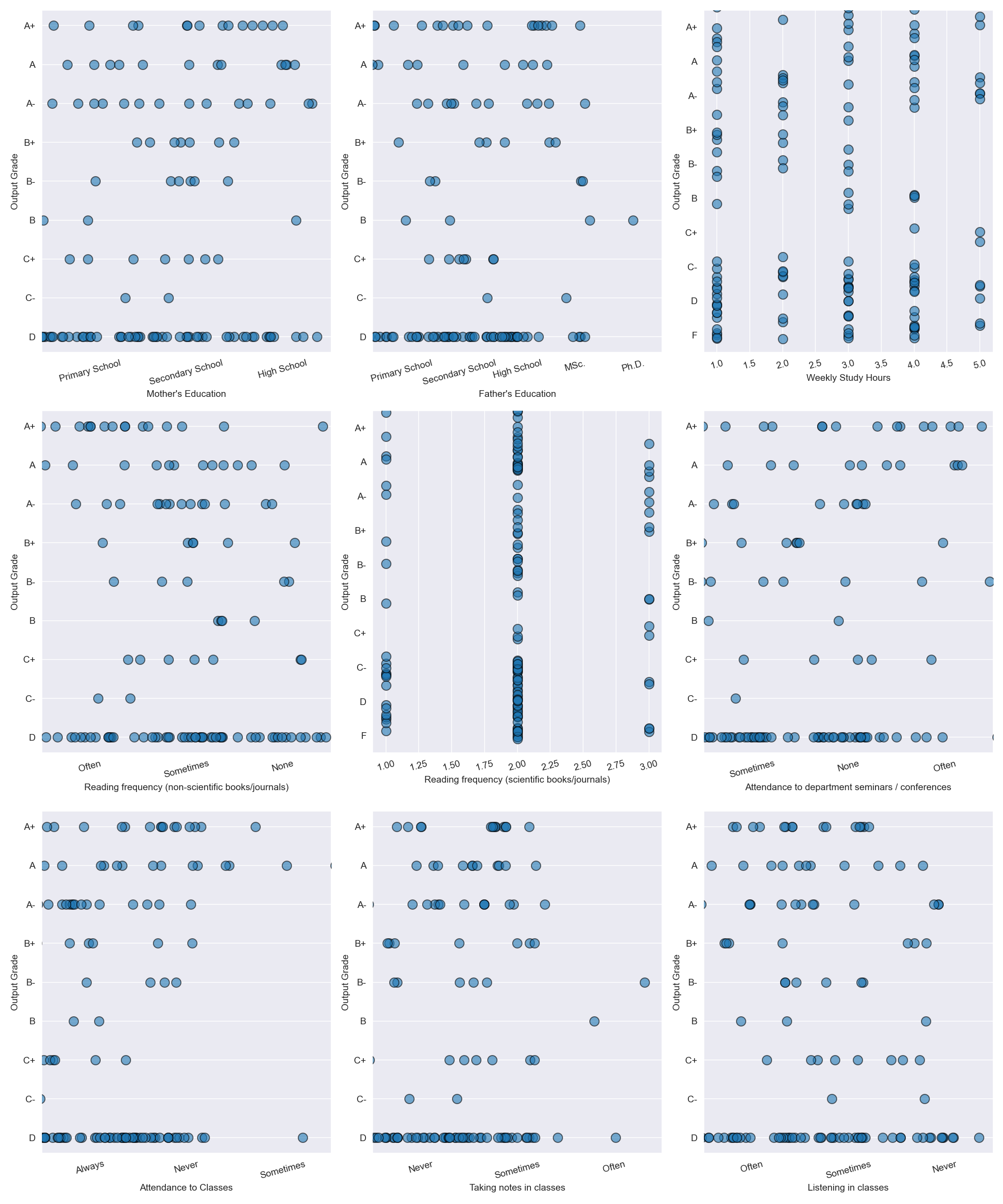
Now, we need to get an idea of which features are particularly pertinent to student success. I have a few initial ideas (such as parent education, how often they attend classes, and how often they listen in classes), but I have no idea which factors high-performing students are doing the most. So I created a series of seaborn swarmplots to help me with this; swarmplots are the best pick here over a traditional scatterplot as much of the data we have overlaps with one another and we need to add a bit of jitter to fully see the data (which is especially helpful given we don’t have an overwhelming number of observations here, which swarmplots struggle with). We can apply some more pre-processing before using the swarmplot to make the axis titles make a bit more sense (previously, they were solely numerical values and I have no idea what a 3 in Mother’s Education means), and then make a subplot of each relevant feature against our target—a student’s grade—to visualize which features might be worth really analyzing!
III. Model Selection
Given that our data is not very linear at all (we can see that with the massive amount of overlap between different data points), utilizing a model that does well this type of data is key. With that in mind, I identified the following models as likely the candidates to perform well for a classification task:
- Support Vector Machine with a non-linear kernel function: Support Vector Machines are best when we are not working with linearly separable data, as we are here; it is able to project our data using a kernel function and find a hyperplane that separates our classes in feature space. They are not the most interpretable machine learning model out there, but they are powerful and versatile to a wide domain tasks (hopefully including ours!)
- Random Forest: Random Forests are an incredibly popular and powerful ensemble model that conglomerates multiple weak decision trees together to create a model that is overall much more accurate and robust. These slew of decision trees mean they can usually provide high accuracy and also provide some awesome insight into the most vital features of our dataset, but unlike their little siblings the Decision Tree, they are not nearly are interpretable or computationally inexpensive, and can also be suspectable to bias to overrepresented classes.
- Gradient Boosting Machine: Gradient Boosting is yet another ensemble algorithm like Random Forest, but it takes a step further by building upon previous models sequentially and correcting the errors of each predecessor. It shares many of the same benefits of Random Forests but with the added benefit of really handling weird datasets well, such as data that is missing or needs to be robustly pre-processed before using it. However, it can overfit and also takes quite a bit of resources to hyperparameter tune (I also don’t understand it as well as the others).
With those models identified, let’s go to implementing them!
IV. Model Implementation
IV.I: Splitting our Data
Before implementing any models, we have to first divide our dataset into a series of training and test datasets. To do this, we can utilize the nifty train_test_split function from Scikit-Learn’s model_selection module. Before I split my data, I also dropped features that I didn’t feel like the model should use for classification (such as gender and age) and those that overlap with our main criteria for student success (output grades), such as expected GPA at graduation.
X = edu_df.drop(columns = ['Age', 'Sex', 'School Type', 'Student ID', 'Parental Status', 'Has Partner', 'Output Grade', 'Expected GPA at graduation', 'Cumulative GPA last semester'])
y = edu_df['Output Grade'].to_numpy()
Also, given the huge skew we saw in the grade distribution during our data visualization, I opted to utilize the stratify parameter with train_test_split to ensure that classes were equally represented in both our training and testing dataset, hopefully giving our models the best chance to not overfit and make good predictions on the test dataset!
# Opting for a slightly bigger test size here given our smaller dataset along with stratifying given the heavy skew in grades that we saw with the previous visualization
X_train, X_test, y_train, y_test = train_test_split(X, y, test_size=.3, random_state = 11, stratify = y)
IV.II: Evaluation Metrics
To see our model performed, we need a way to quantitatively score it. For this, I utilize a series of built-in functions from Scikit-Learn to calculate accuracy, F1-Score, and Confusion Matrices. Accuracy is the default calculation when doing something like this, and is always a helpful metric to have, but in an imbalanced dataset like this, can be highly misleading. If our model does overfit and assigns almost every student a D grade (foreshadowing), then our accuracy might be OK but the few students that do have higher grades will be completely overshadowed! For that reason, I also decided to include a weighted F1-Score to ensure that both Precision and Recall are included within our evaluation, and we aren’t applauding a model that in reality is pretty terrible. Finally, our confusion matrix can provide some great insight into how the model is classifying various how it should be classifying by showing us the predicted class versus the actual class, so if it does make a mistake, we can see which class it is from. Again, many of the metrics are already provided by Scikit-Learn, but I did make wrappers for each so I could just generalize them a bit easier:
from typing import Any

def accuracy_calc(model: Any, X_test: np.ndarray, y_test: np.ndarray) -> float:
    """Calculates the accuracy for a given model on a test set

    Args:
        model (Any): Provided Scikit Learn Model to test with
        X_test (np.ndarray): Test Input for Model
        y_test (np.ndarray): Test Target for the model

    Returns:
        float: Model accuracy
    """
    return accuracy_score(y_test, model.predict(X_test))

def f1_score_calc(model: Any, X_test: np.ndarray, y_test: np.ndarray) -> float:
    """Calculates the f1-score for a given model on a test set

    Args:
        model (Any): Provided Scikit Learn Model to test with
        X_test (np.ndarray): Test Input for Model
        y_test (np.ndarray): Test Target for the model

    Returns:
        float: Model f1-score
    """
    return f1_score(y_test, model.predict(X_test), labels = np.unique(edu_df['Output Grade']),  average = 'weighted')

def confusion_matrix_calc(model: Any, X_test: np.ndarray, y_test: np.ndarray) -> GT:
    """Calculates and visualizes the confusion matrix for a given model on a test set

    Args:
        model (Any): Provided Scikit Learn Model to test with
        X_test (np.ndarray): Test Input for Model
        y_test (np.ndarray): Test Target for the model

    Returns:

    """
    # Get predictions and compute confusion matrix
    cm = ConfusionMatrixDisplay.from_estimator(model, X_test, y_test)

    return cm
IV.III: Naive Implementation
Finally onto making and implementing our models! As any good Machine Learning Engineer would do (right?), after splitting my data and creating my evaluation metrics, I just throw my data to my model with essentially no other tuning or customization. The results, were um, not great.
        svc = SVC(random_state = 11, kernel = 'rbf', degree = 11)

        svc.fit(X_train, y_train)
        print(f'Accuracy Score: {accuracy_calc(svc, X_test, y_test)}')
        print(f'F1 Score: {f1_score_calc(svc, X_test, y_test)}')
        svc_cm = confusion_matrix_calc(svc, X_test, y_test)
        rf = RandomForestClassifier(random_state = 11, max_depth = 7)
        rf.fit(X_train, y_train)
        accuracy_score(y_test, rf.predict(X_test))

        print(f'Accuracy Score: {accuracy_calc(rf, X_test, y_test)}')
        print(f'F1 Score: {f1_score_calc(rf, X_test, y_test)}')
        rf_cm = confusion_matrix_calc(rf, X_test, y_test)
        gb = GradientBoostingClassifier(n_estimators = 150, learning_rate = .15, max_depth = 1, random_state = 11)
        gb.fit(X_train, y_train)
        accuracy_score(y_test, gb.predict(X_test))

        print(f'Accuracy Score: {accuracy_calc(gb, X_test, y_test)}')
        print(f'F1 Score: {f1_score_calc(gb, X_test, y_test)}')
        gb_cm = confusion_matrix_calc(gb, X_test, y_test)
      Accuracy Score: 0.4772727272727273
      F1 Score: 0.32756132756132755
      Accuracy Score: 0.4772727272727273
      F1 Score: 0.32756132756132755
      Accuracy Score: 0.4772727272727273
      F1 Score: 0.42273533204384267
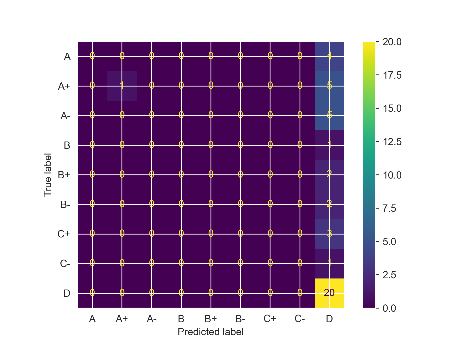
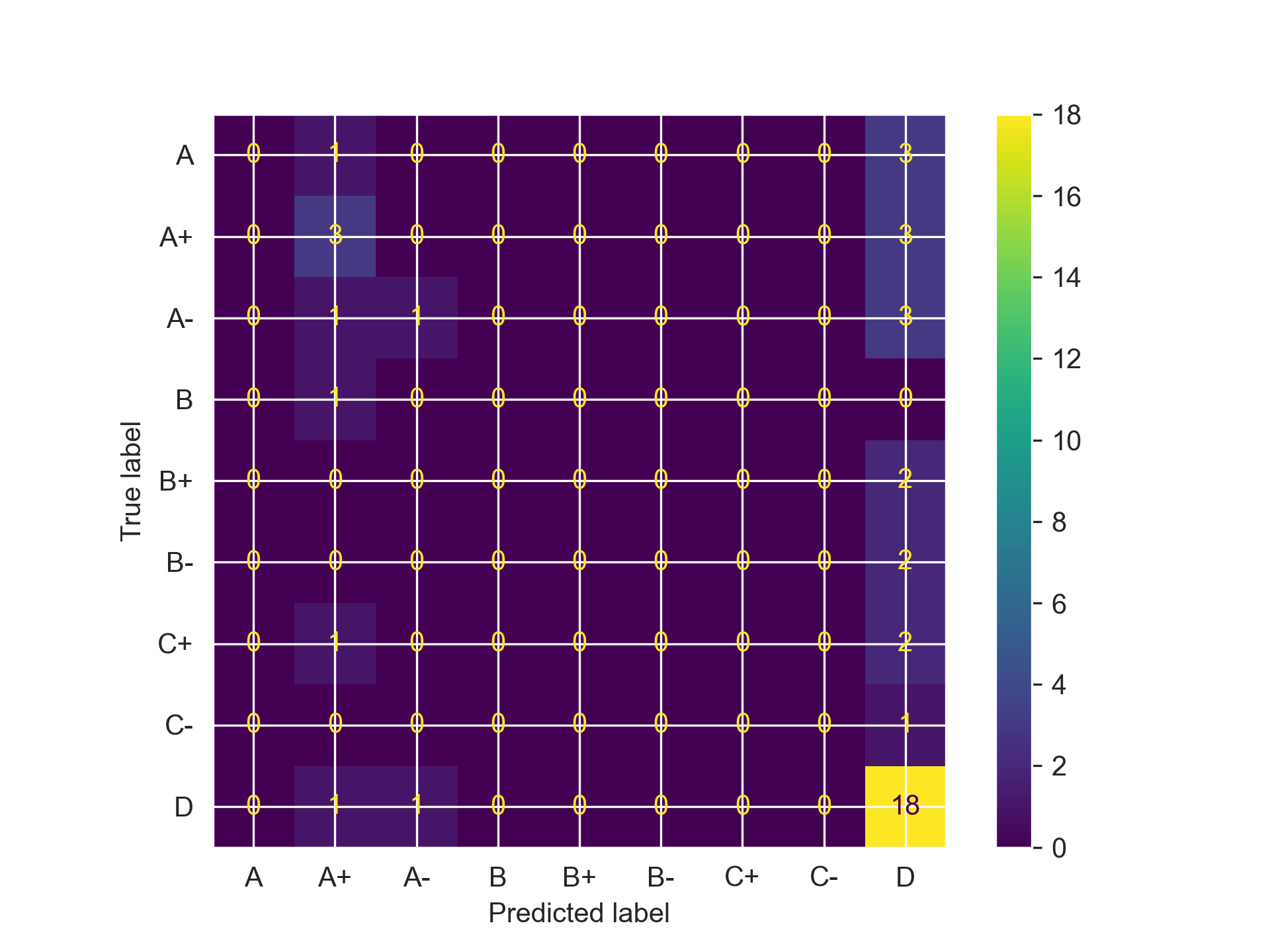
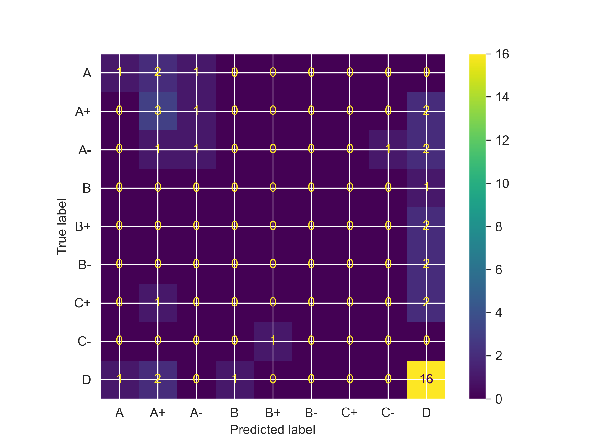
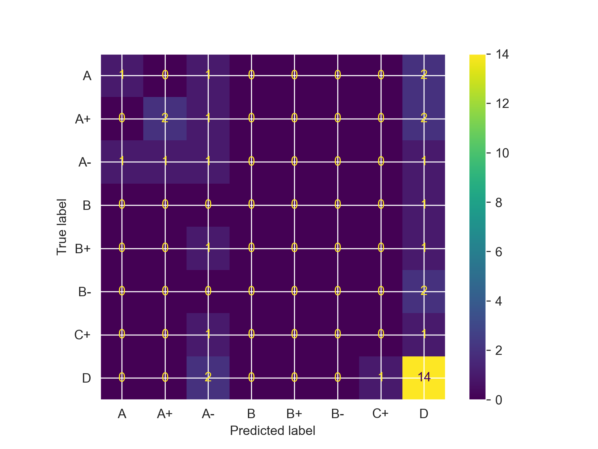
Taking a look at the confusion matrices, we can see that all three models do what I feared: categorizing almost every student as having a D grade, regardless of what the features indicated. They need some serious refinement if they want to actually become usable for anything practical. We can start by reducing the number of features that each utilizes.
IV.IV: Feature Engineering
While I love this dataset and all of the information it provides about students, it’s clear that not all of it is pertinent to accurately predicting student performance and in many cases, might be hurting it. Thus, we need to see which features models are utilizing and focus on those instead of muddying the water with unnecessary noise. Luckily, random forests have a class attribute that can provide us that exact information:
feature_importances: pd.Series = pd.Series(rf.feature_importances_, index=X.columns)
most_important_features: list = feature_importances.sort_values(ascending=False).head(7).index

print(f'The most important features are: {most_important_features}')
The most important features are: Index(['Impact of projects / activities on your success', 'Additional Work',
       'Number of Sisters / Brothers', 'Mother's Education',
       'Reading frequency (scientific books/journals)', 'Weekly Study Hours',
       'Father's Education'],
      dtype='object')
Just looking at these features, a lot of this actually makes a ton of sense. These are engineering students that were surveyed, and that means things like projects and outside activities can provide so much valuable insight and information on the academic development of the participant. The amount of additional work they put outside of classes is vital, and we do see parent’s education does seem to play a role (Mother more than father indicates again the vital role of maternal focus on education in adolescence). The number of sisters and brothers may seem odd, but this is perhaps attributed to having an adequate support system that can aid a student throughout their studies or even having siblings in the same major that provide excellent study aids and peers. Nevertheless, let’s see if focusing on these features can aid our model’s performance. We modify our training and test datasets, and run essentially the exact same code above to get the following:
      # SVM
      Accuracy Score: 0.4594594594594595
      F1 Score: 0.29474757776644567
        # Random Forest
        Accuracy Score: 0.5675675675675675
        F1 Score: 0.5183982683982684
      # Gradient Boosting
      Accuracy Score: 0.4864864864864865
      F1 Score: 0.4370368150855956
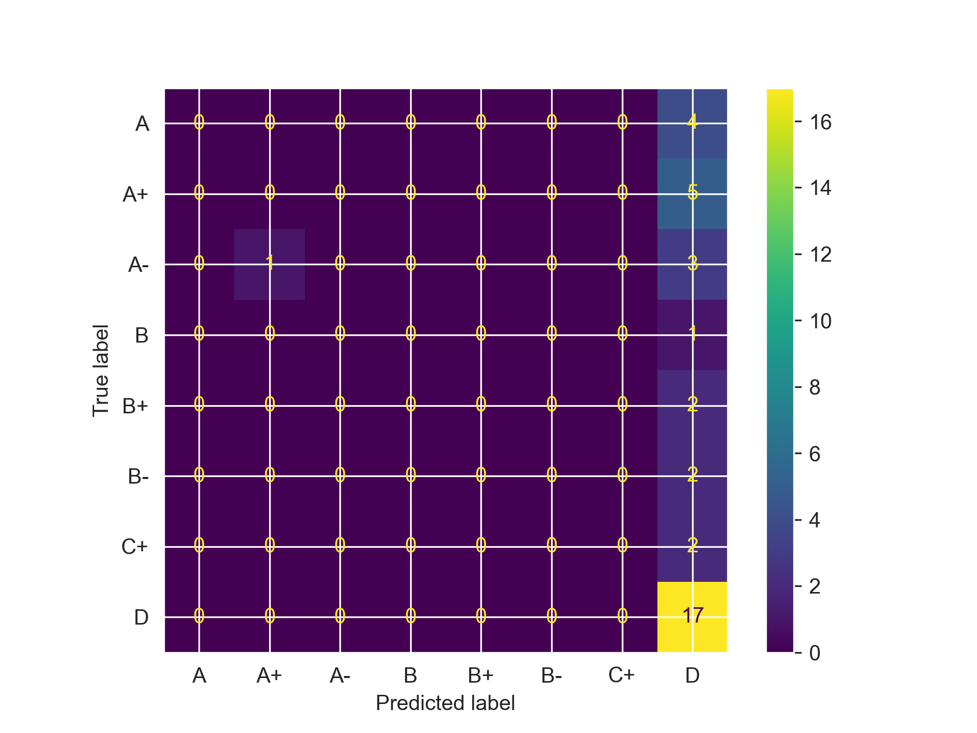
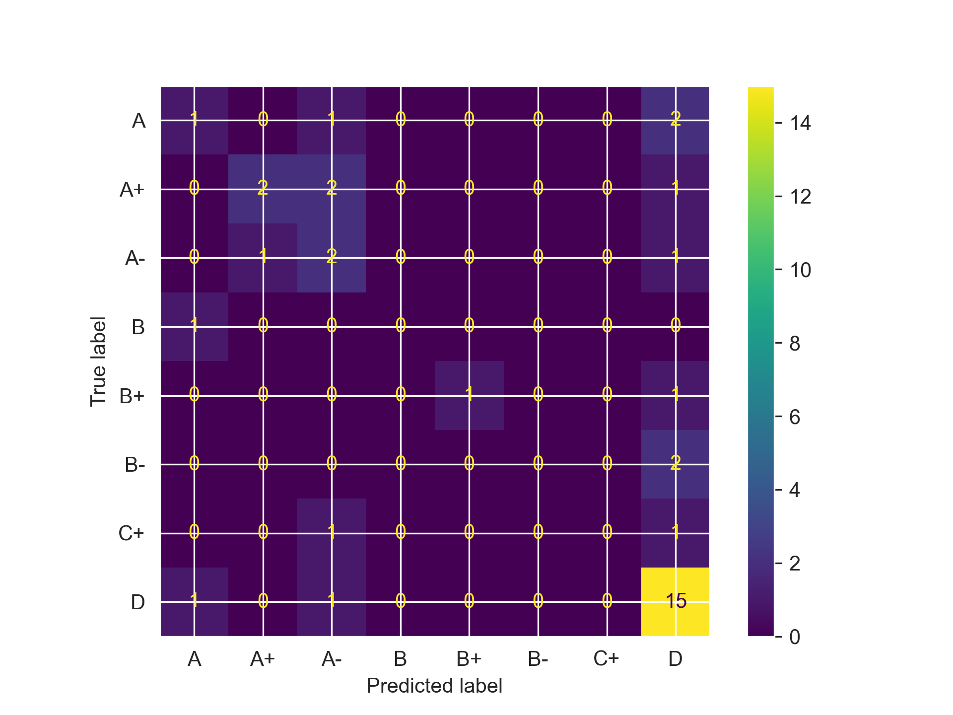
We can see for Random Forest, just focusing on those features provided quite a noticeable accuracy bump, while for Gradient Boosting it minimally improved performance and actually reduced performance for the SVM (oops). Regardless, all of our models are still doing quite poor, meaning we need to try one more thing: Hyperparameter Tuning.
IV.V: Hyperparameter Tuning
Hyperparameters can be incredibly crucial to the performance of every single ML model, so ensuring that they are properly tuned and have the right values is a must. Luckily, Sci-Kit Learn provides a RandomizedSearchCV class that can conduct this entire process for us; all we have to do is define bounds for each hyperparameter and allow Scikit-Learn to take care of the rest. This RandomizedSearchCV is better than the GridSearchCV as it does not search the entirety of hyperspace but randomly queries and tests values for a specified number of iterations, reducing the overall time needed to tune our models. Below is the code for conducting a hyperparameter search for a SVM, but the process is largely the same for Random Forests and Gradient Boosting, just with different hyperparameters and values of course.
# Hyperparameter Tuning for Support Vector

svc_param_grid = {
    'C': [1.0, 2.0],
    'kernel': ['linear', 'poly', 'rbf', 'sigmoid'],
    'degree': [8,9,10,11],
    'gamma': ['scale', 'auto']
}

svc_grid_search = RandomizedSearchCV(
    estimator=SVC(random_state=11),
    param_distributions=svc_param_grid,
    cv=5,
    scoring='accuracy',
    verbose=1,
    n_iter = 11
)


svc_grid_search.fit(X_test_rev, y_test_rev)
svc_rev_hyp = svc_grid_search.best_estimator_

print(f'The best estimator parameters were: {svc_grid_search.best_params_}')
print(f'Accuracy Score: {accuracy_calc(svc_rev_hyp, X_test_rev, y_test_rev)}')
print(f'F1 Score: {f1_score_calc(svc_rev_hyp, X_test_rev, y_test_rev)}')
svc_rev_hyp_cm = confusion_matrix_calc(svc_rev_hyp, X_test_rev, y_test_rev)
And finally, we were able to get some solid results with this:
      # SVM
      The best estimator parameters were: {'kernel': 'rbf', 'gamma': 'auto', 'degree': 11, 'C': 2.0}
      Accuracy Score: 0.8648648648648649
      F1 Score: 0.8517859965228386
        # Random Forest
        The best estimator parameters were: {'n_estimators': 100, 'max_depth': 7, 'criterion': 'log_loss', 'class_weight': 'balanced_subsample', 'bootstrap': True}
        Accuracy Score: 0.972972972972973
        F1 Score: 0.9752661752661753
      # Gradient Boosting
      The best estimator parameters were: {'subsample': 1.0, 'n_estimators': 100, 'max_depth': 4, 'learning_rate': 0.05, 'criterion': 'friedman_mse'}
      Accuracy Score: 0.43243243243243246
      F1 Score: 0.37537537537537535
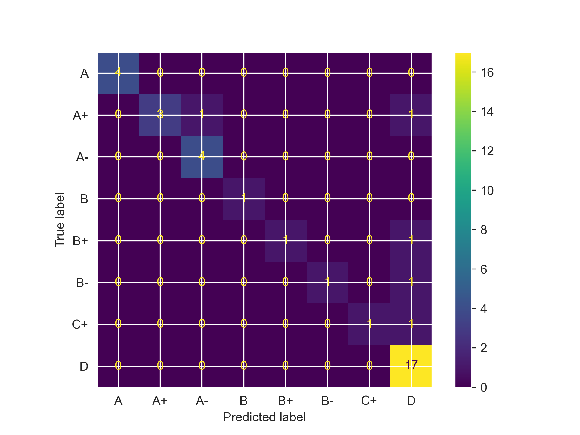
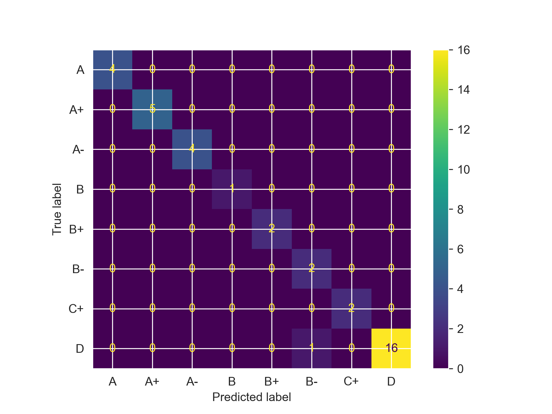

Now, let’s address the elephant in the room before proceeding: yes, I still can’t figure out the Gradient Boosting Trees. Somehow the accuracy got worst throughout the refinement process, and I chalk that up to my own ignorance and novice to the concept, not the model itself (I’ve heard wonderful things about that). However, the accuracy jump for SVMs and Random Forest is incredible, with the latter really doing exceptional across all of our metrics, with only misclassifying one student that got a D as a B- (we just have a nice, overly optimistic model). I knew hypermeters were important, but I’d be lying if I told you I thought the performance would increase this much. We have actually have something that is usable for a potential school setting!
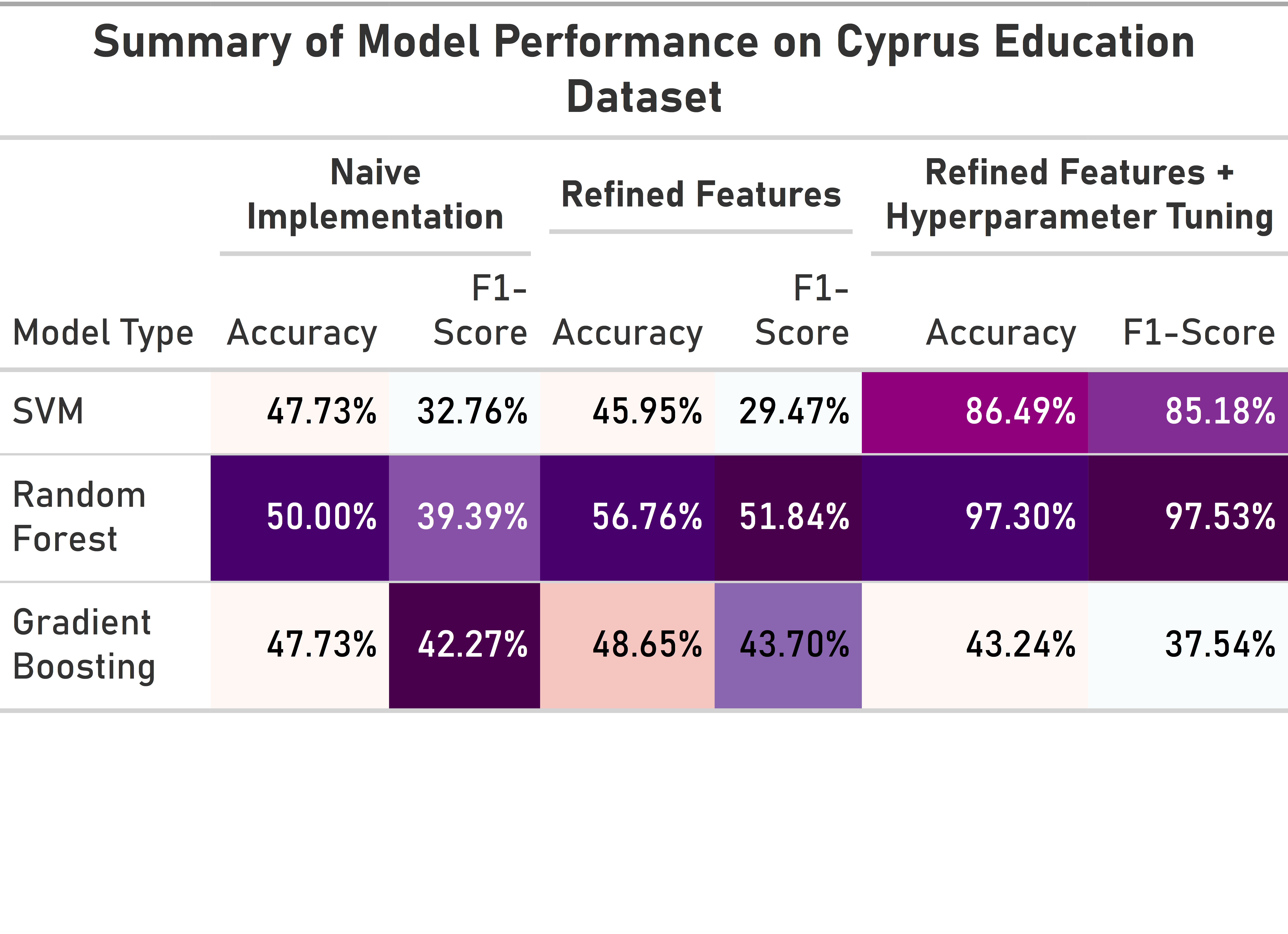
Just to summarize, here all of the results of our models and implementations in a nice table (shout out again to great_tables).
V. Conclusion and Impact
Just to remind you, we set out to answer two main questions: Which features of a student are most correlated with academic success and how can we utilize these features to predict which grades they will achieve in their studies?. We definitely answered both, with our process highlighting the importance of practical hands-on experience outside the classroom, parental education level, and also the need for emotional factors like a support system that can provide comfort and aid. We also found that by focusing on these features, we can accurately predict student grades with an accuracy upwards of 97%, albeit also sometimes as low as 43%. As educators begin to try to implement holistic educational curriculums, focusing on factors like these can help identify inequities before they become systemic an ensure that students are receiving the help needed based upon their own personal situation and lifestyle. Even if these models will forever always be inherently flawed and not a comprehensive predictor of academic success, they can provide a good baseline to identify where students are expected to perform and how they either exceed those expectations——indicating effective instruction and collegiate support—or faltered below them—indicating a need for more robust interventions and overhaul of existing systems.
VI. References
GeeksForGeeks: Comprehensive Guide to Classification Models in Scikit-Learn
GeeksForGeeks: How to Tune Hyperparameters in Gradient Boosting Algorithm
Literally Every Page in the Scikit-Learn Documentation for every model or function I used